Summary: I describe a research project that attempts to estimate a relative height map of the Moon’s surface from a single orbital photograph. No stereoscopy, no machine learning — just classical shadow analysis, brightness gradients, and georeferenced data.

---

The Problem: 3D from 2D

Every photograph of the Moon’s surface is a projection of 3D onto 2D. The elevation information gets “flattened.” To recover it, we have a few clues at our disposal:

• Shadows — the longer the shadow, the taller the object (given known illumination parameters)
• Brightness gradients — abrupt changes in brightness indicate slopes
• Albedo — surface material also alters brightness, which complicates both of the above

The problem is that albedo and topography are entangled. A bright patch in an image could be a plain made of bright regolith or a slope tilted toward the Sun. There is no way to fully separate them from a single frame — this is a fundamental physical limitation. The project openly acknowledges this and builds its entire confidence system around that constraint.

---

Pipeline Architecture

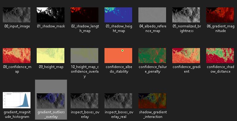
The code is divided into 7 stages, each producing its own diagnostic image:

Stage 1 — Shadow Detection

The shadow mask is generated using a percentile method (default: the darkest 15% of pixels) or a standard deviation method. This is a heuristic approach — dark material may be incorrectly classified as shadow.

01_shadow_mask.png

Stage 2 — Heights from Shadows

Shadow lengths are measured from the shadow mask and converted into relative heights:

height = shadow_length_px × pixel_scale_m × tan(sun_elevation°)

The assumption is that shadow-casting objects are vertical. This is an approximation, but sufficient for rocks and crater rims.

02_shadow_length_map.png
03_shadow_height_map.png

Stage 3 — Albedo Map

The algorithm interpolates “expected” background brightness from so-called inspect boxes — small windows that sample material brightness at known geographic points. In version 2.6, the positions of these boxes are derived from actual lunar coordinates (lat/lon) from QuickMap data, not placed randomly.

04_albedo_reference_map.png

Stage 4 — Brightness Normalization

Observed brightness is divided by the expected albedo brightness to isolate the effect of topography:

normalized = observed / expected_albedo

05_normalized_brightness.png

Stage 5 — Gradients

Spatial gradients (magnitude and direction) are computed on the normalized brightness. A strong gradient indicates a slope; the gradient direction reveals slope orientation.

06_gradient_magnitude.png
07_gradient_direction.png  ← HSV visualization: hue = direction

Stage 6 — Confidence Map

This is the heart of the project. The confidence map combines 5 independent components:

Component	What It Measures
Shadow distance	Proximity to shadow edges
Gradient	Brightness gradient strength
Texture variance	Local variance (texture)
Albedo stability	Proximity to inspect boxes
Failure penalty	Penalty for areas inherently unsuitable for analysis

Final confidence map = weighted sum of components × failure region penalty.

08_confidence_map.png  ← green = high confidence, red = low

Stage 7 — Final Height Map

Heights from shadows and gradient-based slopes are combined. In low-confidence areas, results are smoothed toward the median — to avoid presenting noise as terrain.

09_height_map.png
10_height_map_confidence_overlay.png  ← heights + confidence as opacity

---

Input Data: QuickMap

The project uses data from QuickMap (LROC, Arizona State University):

• LROC NAC image — a high-resolution orbital photograph (~1 m/pixel at full resolution)
• Region Data CSV — measurement points from QuickMap containing: geographic coordinates (lat/lon), terrain height (TerrainHeight), slope (Slope), optical composition, and more

A .vrt file (GDAL Virtual Dataset) provides georeferencing metadata: coordinate system, geographic transform, and pixel scale.

---

Project Iterations

The code went through three iterations, each adding a new layer:

Iteration 2 — basic pipeline (shadows + gradients + confidence map)

Iteration 2.5 — diagnostic layer: confidence map breakdown into 5 components, gradient histogram, outlier overlay, shadow–gradient interaction. Goal: *”Am I trusting the pipeline for the right reasons?”*

Iteration 2.6 — real coordinates: inspect boxes placed using QuickMap data instead of randomly. Lat/lon → pixel mapping via linear approximation (no cartographic projection correction).

Iteration 3 (validate_iteration3.py) — trend validation: comparison of gradient directions against an external DEM (LOLA/LROC). No optimization — it only answers the question: *”Are the reconstructed trends consistent with actual topography?”*

---

What the Project Does Not Do

This list is just as important as the feature list:

• Does not generate a DEM — heights are relative, with no absolute reference
• Does not use machine learning — every step is human-interpretable
• Is not photogrammetry — no stereo pairs, no triangulation
• Does not work well on plains — uniform areas produce no topographic signal
• Does not fully separate albedo from topography — this is impossible from a single image

---

Results and Validation

When tested on a sample lunar region (7.63°N, 6.53°E), at full LROC NAC resolution (1 m/px), using a synthetic DEM (no access to LOLA during testing), Iteration 3 validation classifies:

• approximately 3.6% of high-confidence areas as consistent with the DEM trend
• approximately 17.7% as inconsistent
• the rest: too low confidence to draw conclusions

The results are reported honestly — the project does not attempt to explain away or “fix” these numbers. Inconsistency is information, not an error to be hidden.

---

Potential and Applications

It is worth mentioning the broader context of the data this project relies on.

The images of the Moon’s surface captured by LROC NAC represent the most detailed mapping of a celestial body’s surface beyond Earth. At a resolution of ~1 m/pixel, each pixel corresponds to one square meter of surface area — a level of detail unmatched for any other planet or moon in the Solar System. The absence of a lunar atmosphere eliminates blurring and optical distortions, further enhancing image quality.

QuickMap also offers a 3D view reconstructed from LOLA (LRO Laser Altimeter) data. It provides an extended sense of terrain shape, but like this pipeline, it presents topography within a limited scope — it is not full, precise photogrammetry.

What Else Could Be Extracted

The main limiting premise of this project is a single image from a single angle. If two or more images of the same area were available at comparable resolution and different illumination angles, the analytical possibilities grow significantly:

Traversability assessment — identifying terrain with minimal slope and few boulders, useful for planning rover routes.

Regolith thickness estimation — boulder shadows and their relationship to the surrounding area may indicate the depth of the loose surface layer.

Rock formation analysis — the distribution and morphology of boulders under different illumination angles allows for preliminary lithological classification.

All of this is still research territory, not a ready-made tool. But the starting point is exceptionally good: the data is public, free, and of the highest possible quality.

---

Code and License

The Python code (~1,600 lines, no external AI frameworks) uses only: numpy, opencv-python, scipy, matplotlib

The source code is publicly available on GitHub: github.com/MarcinSFox/Lunar_2.5D

All steps are explicit and documented. Each stage generates its own diagnostic image, making it possible to understand where the pipeline works well and where it fails.

Test data: sample lunar region (~7.63°N, 6.53°E), LROC NAC image from QuickMap, scale ~1 m/px.

---

I treat this project as a research experiment and a learning tool. The results are hypotheses about terrain shape, not measurements. The project’s value lies in the transparency of the method and the explicit modeling of uncertainty — not in the accuracy of the results.